Slide By Sensing for Long Stroke applications using Allegro Angle Sensors

Download PDF Version

 

Abstract

This application note is a guide through the design process for using angle sensor ICs for linear position sensing, including magnet choice and orientation, output linearization, and using sensor IC arrays for extending the measurement range. Test data from a number of magnets and sensing lengths is also provided to show how well the theoretical and real-world accuracy of these solutions match.

Introduction

Accurate, low-cost, and non-contact linear position sensing is often accomplished using a bar magnet and a magnetic sensor IC or array of sensor ICs. The magnet is attached to the moving object, and the sensor is positioned such that the magnet slides by it. The typical configuration and fields seen are shown in Figure 1. As the magnet slides by in the x direction, the field in the y direction looks like a sine wave with the magnetic field versus position being linear around x = 0.

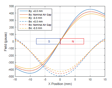
Figure 1: Magnetic fields vs. Position of a bar magnet for multiple air gaps. Magnet length is drawn to scale in all plots.

There are a few challenges to this approach of linear position sensing, including:

• Air gap changes between the sensor IC and the magnet can cause measurement errors.
• Magnetic strength changing over temperature can cause measurement errors.
• The range of measurement over which the magnetic field is linear with position is limited to around 50% of the magnet length, resulting in the need for magnets which are significantly longer than the stroke being measured.

All three of these issues are addressed by measuring the angle of the magnetic field versus position.

• The field angle versus position is nearly identical with respect to the air gap over a typical variance seen in application. Figure 2 shows that the angle versus position is nearly constant versus position, though it does change some as the air gap tolerance gets larger.
• The field angle is independent of the field strength.
• The field angle is linear versus position over the majority of the magnet length, and with linearization, stroke lengths of 150% or more of the magnet length can be sensed. Figure 3 shows the error versus position over air gap after linearizing to the nominal air gap for both the case where By (magnetic field in the y direction) is measured and the case where magnetic field angle is measured. With the By Method, only 10 mm of stroke with 0.5 mm of accuracy (for a ±0.5 mm air gap tolerance) can be sensed for the 16 mm magnet shown. However, with the Angle Method, more than 30 mm of stroke with ±0.5 mm of accuracy can be sensed for the same physical configuration, essentially tripling the linear sensing range.

The Allegro A1335 magnetic angle sensor IC is wellsuited for linear position sensing using the Angle Method described above, as it provides advanced features beyond accurate angle measurement, such as:

• Piecewise linearization of the angle measurement: This allows compensation for the nonlinearity of the angle versus position curve near the ends of the magnets, extending the linear sensing region beyond the edges of the magnet. This also allows for adjustment of the slope of the angle output versus position to any desired value.
• Addressable I²C/SPI/SENT: This allows for multiple ICs in an array to be on the same bus.
• Angle output clamps: This feature is useful for systems using multiple ICs, as clamps can be used to help the MCU to recognize which sensor ICs are out of range and which should be used for determining the position.

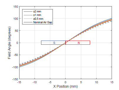
Figure 2: Magnetic Field Angle vs. Position of a Bar Magnet for Multiple Air Gaps.

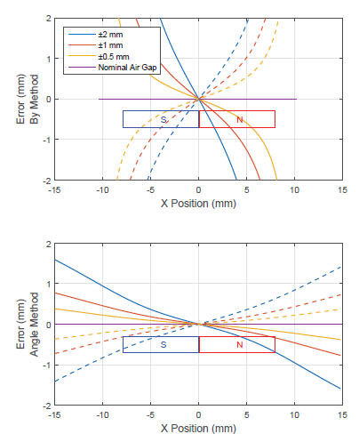
Figure 3: Error vs. Position for By Field and Angle Sensing after Linearization at Nominal Air Gap.

Basic System Configuration

The A1335 is available in a TSSOP-14 package (or dual-die TSSOP-24 for systems needing redundancy) and measures the angle of the magnetic field in plane with the package. This means that for linear position sensing, the IC needs to be oriented perpendicular to the magnet motion, as shown in Figure 4. The effective air gap is the distance from the center of the magnetic sensing array (Circular Vertical Hall sensor) to the edge of the magnet. The CVH is off-center in the A1335, so that can be used to help increase or decrease the air gap in the system as needed.

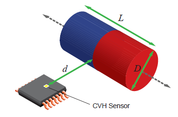
Figure 4: System Configuration using A1335

Designing the Magnetic System for Linear Sensing

The appropriate magnet size and nominal air gap must be chosen for the stroke length being measured to create a system with the desired accuracy. Mainly, the system needs to be designed such that:

• The magnetic angle is generally linear with position.
• The magnetic angle is constant enough versus the air gap tolerance of the system.
• The magnetic field strength is above the minimum needed for CVH based sensor ICs, which is around 300 gauss.

While this seems like a lot to balance, there are a wide range of magnetic systems which will work for a particular application, and each variable in the magnetic system has a specific impact on the accuracy, allowing adjustments to be made quickly to improve performance, reduce cost, etc.

• Magnet Length (L): As a rule of thumb, the magnet length should be at least 60% of the stroke length. The linearity and accuracy over air gap tolerance degrade farther past the edge of the magnet, so, in general, the longer the magnet is, the lower the error will be for a given stroke length.
• Nominal Air Gap (d): The air gap needs to be chosen such that the angle versus position is nearly linear. With really small air gaps, especially on longer magnets, the x and y fields will become non-sinusoidal (Figure 5), and the angle versus position will not be linear or as consistent over air gap tolerance (Figure 6). In general, an air gap in the range of L/3 to L/2 works well.
• Magnet Diameter (D): In general, the larger the diameter of the magnet is, the stronger the field will be. Making the diameter roughly equal to or slightly less than the air gap usually works well for neodymium magnets, which are recommended. Ferrite magnets are cheaper; however, as they are around 4 times weaker, a significantly larger magnet would need to be used to achieve the same field level.

Overall, for a given stroke length, L_S, a reasonable design to start with is:

L = L_S × 0.65

d = D = 0.4 × L

From there, these parameters can be increased or descreased in order to meet the goals of the application.

To determine whether the system will meet the design goals, the magnetic fields need to be modeled. While using advanced 3D magnetic modeling software will yield the most accurate result, it is not necessary in most cases. Fields can be modeled accurately enough using free 2D simulation software available online. Alternatively, the fields can be fairly easily computed in the case where a cylindrical magnet is used, and a MATLAB function for doing this is provided in the Appendix. A bar magnet of similar size will result in nearly identical fields. Figure 7 shows the theoretical angle versus air gap for a cylindrical magnet using these equations, as well as the experimental results using the A1335— the two match well.

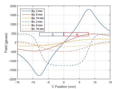
Figure 5: Magnetic Fields vs. Position for a D = 3/8″, L = 5/8″ Magnet at Different Air Gaps

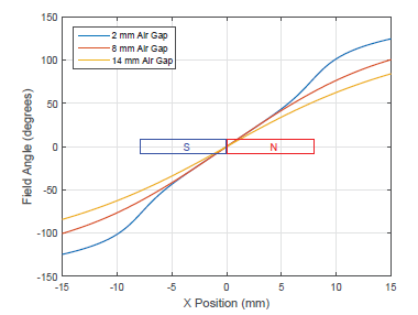
Figure 6: Magnetic Angle vs. Position for a D = 3/8″, L = 5/8″ Magnet at Different Air Gaps

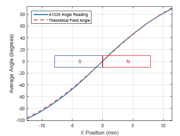
Figure 7: Magnetic Field Angle vs. Position, Theoretical and Measured

Linearization/Calibration Method

Depending on the needs of the system, different linearization or calibration methods may be used. Here, a method for linearizing the output of the A1335 versus position using the Allegro A1335 Samples Programmer is described. This method can be applied to every system, or the results can be used from one system and apply the found coefficients to all the other systems to get similar performance with less impact to test time in production.

• Start Up Programmer: Connect the A1335 to the ASEK20, and connect the ASEK20 to your computer. Start up the Samples Programmer software and power on the A1335. See the Allegro A1335 Samples Programmer User Manual for more details on getting started with the programmer.
• Go to the Long Stroke Tab: The “Long Stroke” tab of the programmer helps automate the process of using the segmented linearization available on the A1335 for linear position applications. It also helps to mask the fact that angle measurements are being dealt with and only works in position.
• Determine the Range of Travel and Codes/mm: The full range for linearization using this method is from code 256 to code 3840, avoiding the range around zero where rollover occurs, so the full stroke needs to fit within this range. That means that the codes/mm value, Cpmm, should be:
  
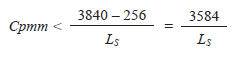
  For example, if the stroke length is 25 mm, Cpmm should be 143.36 codes/mm or less, so that value might be rounded down to an integer value, or perhaps 128, to simplify the math in their microcontroller for converting from codes to millimeters. If the “Range of Travel” is entered as 25 in the Samples Programmer and then clicks the “Calculate mm/ step and codes/mm” button, the Cpmm value will be shown. Then this value can be rounded down to the desired number; after this, click the “Calculate Range and mm/step” button. This will recalculate the “Range of Travel” based on the new Cpmm value. For example, if Cpmm were rounded to 128, the “Range of Travel” would now be 28 mm, which gives a reasonable amount of margin around the desired 25 mm range of measurement.
• Determine mm per Linearization Step: The piecewise linearization points are every 256 codes, so determine how many millimeters to move between each linearization point.
  
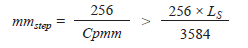
  For the example considered above, mmstep should be greater than 1.79 mm, and since Cpmm was chosen to be 128, mm_step is 2 mm. This value is shown in the Samples Programmer, and the result of this is seen in the data input table as the difference in millimeters between each linearization point.
• Start Linearization Measurements at X = 0: Fill in the measurement table. Essentially, at each “Distance,” measure the raw output of the sensor. After the linearization, the linear transfer function is described by the “Distance” and “Desired” code columns. Start at position X = 0 (magnet is centered on CVH sensor), ensuring that the “Distance” = 0 row is highlighted, and clicking the Read Value button. The “Measured” column will then be populated with the sensor reading, and the highlighted row will shift down.

Continue Linearization Measurements: Step in position by mm_step, reading the sensor output into the correct row of the table. The process is as follows:

N = 1

Step to position X = N * mm_step.

Make sure the row for X = N * mm_step is highlighted. The software will increment/decrement the row after each read, leading through the measurements.

Click the “Read Value” button to read the value from the A1335 and populate the measurement value in the highlighted row.

Repeat steps b through d, incrementing N each time until N = 7.

Repeat steps b through d, except N now goes from –1 to –7.

Calculate and Apply Coefficients: Click the “Calculate and Program Device” button. This will calculate the correct values for the offset and linearization and program them to the device. Check the Performance: Click the “Start Test” button to constantly read out the position from the sensor. Then move the magnet and check the reading from the sensor. An example of a linearized sensor output is shown in Figure 8. Here, the position was changed 2 mm for each linearization point, mm_step = 2. This means that Cpmm = 256/2 = 128 codes/mm, which is the slope of the sensor output after linearization, as seen in Figure 8. Also, at position X = 0, the sensor outputs 2048. Figure 8: Linearized output of A1335 over Air Gap. Magnet 1. Experimental Results for Multiple Magnets and Stroke Lengths Linearization results are provided below for three different magnets over different stroke lengths. The key values for each magnet used are given in the table below (all magnets are Neodymium): Magnet Stroke Length mm_step # Diameter Length 1 6.4 mm 15.9 mm 25 mm 2 mm 2 9.5 mm 19 mm 30 mm 3 mm 3 12.7 mm 38.1 mm 50 mm 4 mm The plots below for each magnet show the output angle versus position and the error in the measured position versus position over multiple air gaps. The error is based on the ideal sensor output, which should be: Rearranging this shows how to convert from the sensor output of the A1335 to an X position. The error is then just the difference between the actual X position and the calculated X position from the sensor IC output. For Magnet 1, this error is shown in Figure 9. Figure 9: Measurement Error vs. Position over Air Gap. Magnet 1. Figure 10: Linearized output of A1335 over Air Gap. Magnet 2. Figure 11: Measurement Error vs. Position over Air Gap. Magnet 2. Figure 12: Linearized Output of A1335 over Air Gap. Magnet 3. Figure 13: Measurement Error vs. Position over Air Gap. Magnet 3. Accuracy Over Temperature and Resolution One of the main benefits of using the Angle Method for sensing linear position is that it is highly accurate over both air gap and temperature. The previous sections all dealt with accuracy over air gap. Accuracy over temperature is mainly dependent on the angle accuracy of the sensor used. The accuracy of the A1335 over temperature is around ±1.3 degrees; however, this must be converted to millimeters in the system. As the angle error is relative to the nonlinearized angle output, the raw angles being swept, which is around 180 degrees over the full stroke, must be considered. This can be seen in Figure 2. The error in position measurement can then be calculated as: For a 25 mm stroke, L_S = 25, the error over temperature would be ±0.18 mm. The position resolution can be calculated using essentially the same method. For the A1335, the angle resolution is 0.8 degrees (3 sigma). This means that the position resolution for a 25 mm stroke will be 0.8 / 180 × L_S = 0.11 mm. Of course, if internal filtering of the A1335 is enabled or number of readings are averaged, this resolution will be improved. Extending the Sensing Range using Multiple Sensor ICs Extending the sensing range can be done either by increasing the magnet size, following the guidelines above, or by adding more sensor ICs to the system. As the desired stroke length gets larger, the cost and size of the larger magnet will drive the solution towards using multiple sensors. A configuration using multiple sensors is shown in Figure 14. Here, three sensor ICs are used, but this can be extended to n sensor ICs. Figure 14: System Configuration for using Multiple A1335 Angle Sensors The desired stroke length, L_S, is divided by n (3 in the case of Figure 14) in order to have an effective stroke length, L_seff, of: The magnetic system is then designed around L_seff, using the methodologies described above, and the n sensors are spaced L_seff, away from each other, center to center. Besides making the magnet smaller, this also results in lower error over temperature, as L_S is reduced: As the magnet passes beyond the range of one sensor, it enters the range of the next sensor. Determining which sensor IC to read the position from is fairly simple with the A1335. During normal operation where the position is periodically measured, if the position reading from the sensor currently being used goes beyond L_seff / 2 in either direction, switch to the next sensor over. To avoid switching back and forth between two sensors a lot right at L_seff / 2, some hysteresis can be added to this switchover, waiting for the position to go a little beyond L_seff / 2 before switching. At startup, or after a long period of not reading the position, it may be necessary to determine which one out of the n sensors to use for reading the position. The challenge here is that if n is large, some of the sensors may not have enough field on them to give a valid output. Here, the low field error register of the A1335 can be used to determine which sensor outputs to ignore. Then, of the sensors which are giving valid outputs, the one giving an angle output closest to 180 degrees should be chosen as the active sensor. Conclusion Overall, magnetic angle sensor ICs work significantly better for linear position sensing than single-axis magnetic sensor ICs. The Allegro line of CVH-based angle sensor ICs, such as the A1335, are well-suited for these applications, providing advanced features, such as piecewise linear (PWL) linearization and addressable SENT, I²C, or SPI, which help extend the usable sensing range from a magnet, and simplifying and reducing the cost of the total system. APPENDIX A: MATLAB FUNCTION FOR CALCULATING FIELD FROM A CYLINDRICAL MAGNET function [Bz,Br] = cyl_field(B,L,Radius,z,r)
% Bz and Br are the Z and Radial direction of the field from a cylindrical magnet
% where B is the residual inductance of the material, L is the length of the
% magnet, and Radius is the radius of the magnet.
% z is the distance from the center of the magnet along the z axis, and r
% is the distance from the magnet in the radial direction.
bz = @(R,phi,z,L,r) R.*(L/2-z)./((R.^2+(L/2-z).^2+r.^2-2*R.*r.*cos(phi)).^(3/2))...
+R.*(L/2+z)./((R.^2+(L/2+z).^2+r.^2-2.*R.*r.*cos(phi)).^(3/2));
br = @(R,phi,z,L,r) -R./2.*(2.*r-2.*R.*cos(phi))./((R.^2+(L/2-z).^2+r.^2-2.*R.*r.*cos(phi)).^(3/2))...
+R./2.*(2.*r-2.*R.*cos(phi))./((R.^2+(L/2+z).^2+r.^2-2.*R.*r.*cos(phi)).^(3/2));
% Fix the field calculation value if one is inside the magnet
if (z <= L/2*1.01) && (z > -L/2*1.01) && (abs(r) <= Radius*1.01)
Bz = B/2;
Br = 0;
else
Bz = -B./(4*pi)*integral2(@(R,phi)bz(R,phi,z,L,r),0,Radius,0,2*pi);
Br = -B./(4*pi)*integral2(@(R,phi)br(R,phi,z,L,r),0,Radius,0,2*pi);
end
end